Bayesian statistics for the gradient-based data scientist

YouTube tech talk is in this link. Code repo is here.

Depending on the stage of your career as a data scientist, Bayesian statistics might have made its appearance in a variety of contexts. Today, being a data scientist has such a wide meaning that, most likely, you’ve found that not knowing Bayesian statistics has not prevented you from doing your job. This might have you wonder why people make such big fuzz about it.

Back in my physicist days, my formation involved statistics but there was never any mention of Bayesian statistics. When I first heard the term my thought was “You mean like Bayes rule? … Sure I know Bayesian statistics.”. When I was finally properly introduced to the topic, I learned that there are two schools of statistics: Bayesian and frequentist. As it was explained to me, the philosophical differences between these two approaches meant that one can ask to a Bayesian stuff such as “Hey, what is the probability that I have a missing twin?” and have a peaceful discussion about it. A frequentist, on the other hand, will presumably scold you for your nonsense question. Understanding the philosophical differences between the two schools of thought was ok, but it didn’t quite take me all the way. It gave me the impression that, if I wished to talk about probability with anyone, I should first ask if they are frequentist or Bayesian, so that I might not say something offensive. It took me a while to understand what the practical implications were. For example, when I’m doing my usual “fit-predict” stuff, am I taking a frequentist or a Bayesian approach? Does it even matter?

I will soon turn 31, and Boy, this post took me a while to write. Anyhow, I feel like adults should somehow act responsibly. This is why I’ve decided to write it all down, so that any data scientist out there that remains confused and too afraid to ask can finally find some peace of mind when it comes to Bayesian inference.

This post will contain some technical stuff. If it feels new to you, I recommend you take your time to digest the ideas. Take pen(cil) and paper and try to do the derivations yourself. I’m sure that even if you never need to apply Bayesian statistics to your workflow directly, simply understanding the topic will give you a whole new perspective that will strengthen your intuition about the things you already know.

What is Bayesian Statistics?

Let’s put it all into context. Recall that we care about 2 things in data science:

1. Estimating parameters of a model, and
2. Making predictions about unobserved data.

If you’ve been xgboosting all over the place, maybe you no longer care about the specific parameters that optimized your model, but you still care (I hope) about point 2. In Bayesian inference, one applies Bayes rule to the relationship between parameters, \(w\), and data, \(D\). In case you need a reminder, here’s what it says:

This is where a frequentist is meant to jump out of the bushes and try to shame you in front of all your friends. For a frequentist, parameters are not random variables so they claim it does not make sense to talk about its probability distributions. This first came as a surprise to me because any well trained mathematician knows that one does not need “randomness” to talk about probability measures. In any case, Bayesians are kinder creatures that use distributions to quantify uncertainty. Is the Bayesian point of view correct? Yes, but that’s the wrong question. The correct question is what is it useful for?. The Bayesian approach will differ from traditional ML in 2 important aspects:

1. In traditional ML, we use regularisation to control the values of the parameters in your model. In the Bayesian approach, domain knowledge is used to select a prior distribution for the parameters.
2. In traditional ML, we make predictions using the “best-fit” values of the parameters. In the Bayesian approach, predictions are made using all of possible values of the parameters that are consistent with the data.

We will cover these two points in this blog. But first, I need to put a toy example in your head.

A toy example and its Bayesian interpretation

This is how a typical workflow looks like in ML. Say we are given a binary classification task, \(\left\{x_i, y_i\right\}_{i=1}^{N}\), with the dataset below, where the have label \(y=1\) and have \(y=0\).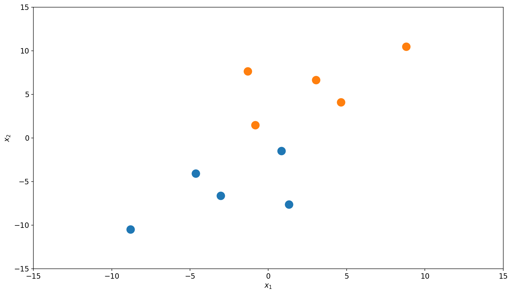

We refrain from taking out our xg-hammer this time and use simple logistic regression:

The plot below shows the classification boundaries, with and without regularisation. I think we can both agree that the plot on the right “looks” better. The plot on the left has a very tight boundary which is not very reasonable. Why? Because you have some experience with logistic regression, so you know that a tight boundary is the result of large weights. But very large weights (anything above 5) are very rare in real life logistic regression. This is why it never crossed your mind to not regularise your logistic regression (right?). In fact, even if you forgot, the developers of scikit-learn got your back: regularisation is included by default on the scikit-learn implementation.

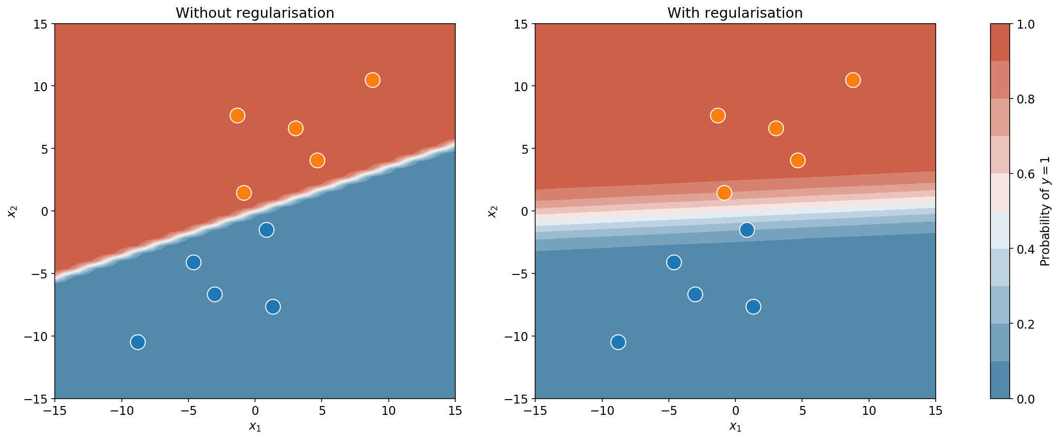
Now, even with regularisation, there’s something that you should still feel uneasy about. Take a second look at the plots above. Notice how, in both cases, the classification boundary extends to the left and right in a straight line. Far away from the data or close to it, the boundary is just as tight. Now take a good hard look at yourself, you know that can’t be right.

Bayesian interpretation

To understand how we are going to fix this unsettling issue, we are going to need a change of perspective about the way we train our models in the first place.

Remember that in logistic regression, like in many other ML tasks, your goal is to find the set of weights, \(w\), that minimise a cost function. Let’s call such cost function \(C\). In the particular case of logistic regression, that cost function is

\begin{align} C(y, x, w) &= \frac{1}{2}w^2 + \sum_{i=1}^N (1 - y_i) \log (1 - f(x_i, w)) + y_i\log f(x_i, w), \tag{1}\label{eq:one} \end{align}

where \(f(x , w) = 1/(1 + e^{-x\cdot w})\). In general, we can write the cost function as two terms: a regulariser and an error. The regulariser is a term which depends only on the parameters. It takes large values when the parameter take large values. Thus, its only goal is to prevent the “best-fit” parameters from getting too large. The “best-fit” parameters are mostly decided by the error term, which depends on both the parameters and the data.

If we put on our Bayesian hats, then the above gives a natural probabilistic interpretation to the process of learning. First we interpret the output \(f(x, w)\) literally as the probability that the input \(x\) has label \(y=1\). In other words, \(f(x, w) = P(y=1\vert x, w)\). This can then be used to show that the error term is in fact the negative log-likelihood of the parameters:

Similarly, if we put the regulariser on the same footing, we can interpret it as defining a probability distribution for the parameters:

\begin{align} P(w) = \frac{1}{Z_R}\exp(-R(w)) \tag{4}\label{eq:four} \end{align}

Since there’s no dependence on the data yet, expression \eqref{eq:four} is called a prior distribution. The constant \(Z_R\) is just a normalisation factor to ensure that probabilities integrate to \(1\), but it does not depend on \(w\) so it does not affect the overall shape of the distribution. We don’t need to worry too much about it. By Bayes rule, the cost function then defines a posterior distribution for the parameters¹:

\begin{align} P(w\vert x, y) &=\frac{P(y\vert x, w) P(x\vert w) P(w)}{P(x, y)} \quad\quad \text{From Bayes rule}\newline &=\frac{P(y\vert x, w) P(x) P(w)}{P(x, y)} \quad\quad \text{Assume } P(x\vert w) = P(x)\newline &= \frac{e^{-E(x, y, w)} e^{-R(w)} P(x)}{Z_R P(x, y)} \end{align}

Finally, if we simply define \(Z_C = Z_R P(y\vert x)\), then

\begin{align} P(w\vert x, y) = \frac{1}{Z_C}\exp (-C(x, y, w)). \tag{5}\label{eq:five} \end{align}

And this is the punchline:

The minimum of the cost function is the maximum of the posterior distribution – a.k.a. the mode.

When you fit your model and get a “best-fit” value for \(w\), such value is often called the MAP estimate (for maximum a posteriori²). If we don’t regularise we get \(R(w) = 0\) which in turn would imply that \(P(w) = \text{constant}\), that is, a uniform distribution. In this case, the posterior distribution is equal (up to a constant factor) to the likelihood, and finding the best \(w\) corresponds to finding a maximum likelihood estimate³, a term which I’m sure you’ve heard before. Let’s talk a bit more about that regulariser prior distribution and how it interacts with the posterior.

Prior vs Regulariser

Typical regularisation techniques are often presented as penalties: L2 penalty, L1 penalty, no penalty, etc. In the toy example above, I used an L2 penalty which is a quadratic function of the weights – see \eqref{eq:one}. The idea of penalties is to put a heavy cost on large values of the parameters, which drives the final estimates closer to zero. From the Bayesian viewpoint however, this L2 penalty corresponds, via equation \eqref{eq:four}, to a prior gaussian distribution centered at zero. The effect is the same, but the interpretation is different and, if I may say, more powerful. In the Bayesian framework you’re not limited to use priors that play the role of penalties. A prior distribution is something that you know about your parameters before you see any data. This could be the fact that the weights are small numbers (as is the case of penalties), but you can specify more complex distributions that better reflect your knowledge. For example, you might want to say that a certain parameter is close to \(1\), instead of close to zero. Or maybe, having negative coefficients would not make sense and you want to constraint your parameters to be positive. Or perhaps, you know that parameter \(w_1\) should always be greater than \(w_2\), etc. The Bayesian approach is the way to go when you want to make inferences that respect and exploit your prior knowledge of a subject.

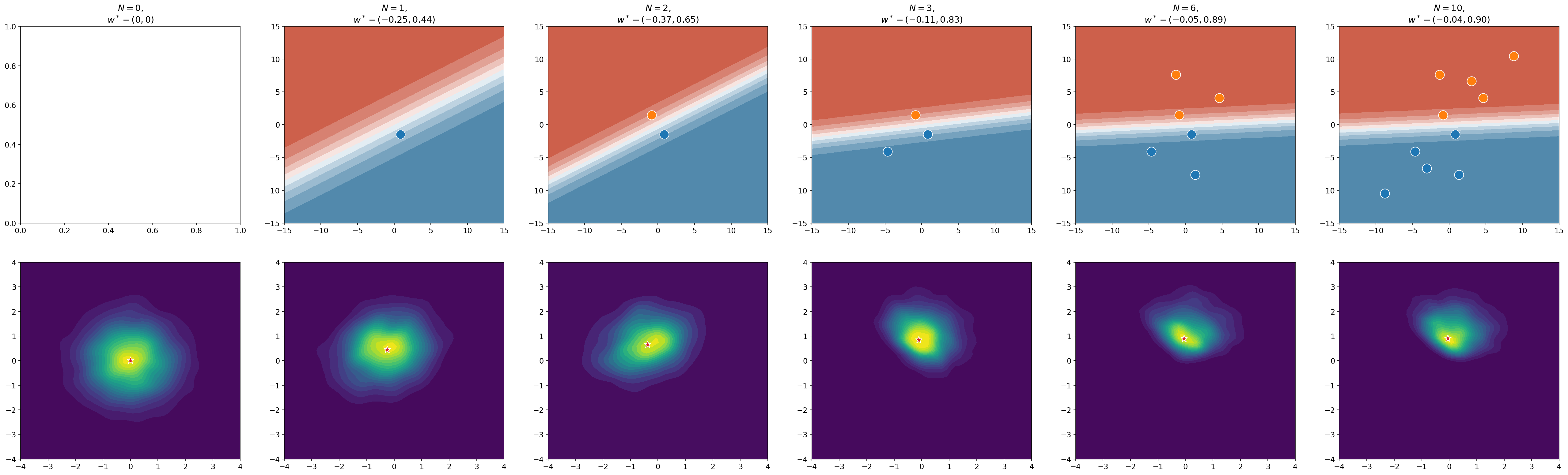
As you collect data, your prior is updated to reflect the fact that you now have more information; it becomes a posterior. The figure below shows an example of what happens to the prior distribution as you see more data. On the far left, you have no data, so the prior is just a Gaussian centered at zero – a Gaussian because you are using L2 regularisation. With each new data point, the distribution moves towards the set of parameters that best describe the data. We now call it a posterior distribution. If you take the mode of that posterior distribution and use it to make predictions, you will get the classification boundary that is shown in the top row of the figure. I’ve marked the mode with a ★.

Making predictions the right way (and the wrong way)

So now that we’ve seen a couple of data points and their labels, we want to make predictions about new data points. What does that mean in probability terms?

1. We have seen data \(x\) with its corresponding labels \(y\),
2. We now have new data \(\tilde{x}\), but no label. We don’t know \(\tilde{y}\).
3. So we ask what is the probability \(P(\tilde{y}=1\vert \tilde{x}, x, y)\) ?.

And this is how you get the correct answer⁴:

\begin{align} P(\tilde{y}\vert \tilde{x}, x, y) &= \frac{P(\tilde{x}, \tilde{y}\vert x, y)}{P(\tilde{x}\vert x, y)}\newline &=\frac{1}{P(\tilde{x}\vert x, y)}\int\mathrm{d}w P(w, \tilde{x}, \tilde{y}\vert x, y)\newline &=\frac{1}{P(\tilde{x}\vert x, y)}\int\mathrm{d}w P(\tilde{y}\vert w, \tilde{x}, x, y) P(\tilde{x}\vert w, x, y) P(w\vert x, y)\newline &=\int\mathrm{d}w P(\tilde{y}\vert w, \tilde{x}) P(w\vert x, y). \tag{6}\label{eq:six} \end{align}

Now, the following might come as a shock to you. You’d hope that whenever you take your trained model and do model.predict_proba(X_test), the above integral is being computed to give you the answer. After all, to compute the integral you need to know the likelihood and the posterior, both of which you’ve already specified. But no. God no. Integrals are difficult and even approximate answers require heavy computation. Instead, the answer you get is simply the likelihood function evaluated at the posterior mode:

\begin{align} \texttt{model.predict_proba(X_test)} &= P(\tilde{y} \vert w_{\mathrm{mode}}, \tilde{x}) \tag{7}\label{eq:seven} \end{align}

This is the wrong answer. The only version of the world in which this answer is correct is if the whole posterior distribution were concentrated in a single point like a Dirac delta distribution. Now, it is true that with more and more data the posterior distribution will indeed get tighter (provided you have adequate regularisation). Despite being technically wrong, using equation \eqref{eq:seven} is often good enough. But the point is that it often isn’t. The main reason to use the answer given in \eqref{eq:seven} (which is wrong) instead of the answer given in \eqref{eq:six} (which is correct) is computation. The mode, \(w_{\mathrm{mode}}\), can be found easily using gradient descent – taking derivatives is easier than calculating integrals.

Suppose now, that you’re not in a rush for once. What would you have to do to compute the correct answer \eqref{eq:seven}? In some cases, the data and model at hand will be simple enough and one will be able to compute the integral analytically⁵. The real challenge is to develop an algorithm that can compute the integral exactly for any likelihood function. Since the likelihood depends on the data, and data comes in all sorts of flavours, this is a very difficult problem. I have a truly marvelous algorithm to do this which the margins of this post are too narrow to contain. So, instead let’s talk about how compute the integral approximately. These are some options:

• Laplace’s approximation.
• Variational inference.
• Monte Carlo methods.

Here I’ll tell you about the last one.

Monte Carlo

Entire books, PhDs, legends, and songs have been written on this topic. Someone even named a casino after this subject. Needless to say, I’ll do no justice to the its complexity. My notes here will be pretty basic– just so that we can keep talking about Bayes. If you’d like to read more about it, I strongly recommend you read this great post by Mike Betancourt.

If you look closely at equation \eqref{eq:six} you’ll notice that the integral that you have to compute has a meaning: it is the average of the likelihood function under the posterior distribution. And we know how to compute the average of something, we just need many samples of it:

\begin{align} \int\mathrm{d}w P(\tilde{y}\vert w, \tilde{x}) P(w\vert x, y) \approx \frac{1}{N}\sum_{i=1}^{N} P(\tilde{y}\vert w^{(i)}, \tilde{x}) \tag{8}\label{eq:eight} \end{align}

where \(w^{(i)}\) is sampled from the posterior, \(w^{(i)} \sim p(w\vert x, y)\). This might seem like a simple solution, but really we just traded one difficult problem for another. We’ve got rid of the integral (so that’s great), but now we need to sample from the posterior (so that’s not great). Lucky for us, this other difficult problem has already been solved by other people.

But, why is sampling difficult? You’ve surely used random number generators before, think of np.random.normal() for example. So the idea of generating random samples from a distribution might sound a like a trivial problem at first. How difficult can it really be to write code for a generic distribution? In fact, if we’re given a random number generator (RNG for short) that follows a uniform distribution in the interval \(\left[0, 1\right]\), then constructing other 1-dimensional distributions is not that difficult. The real problem is constructing RNG’s for high-dimensional distributions. Naively implemented algorithms will at some point require you to evaluate the density over a uniform grid, so they will be extremely inefficient. So inefficient in fact, that they are entirely useless.

If one wishes to generate samples for a high dimensional distribution, the problem has to be approached in a very clever way, evaluating the density only at the places where it really matters⁶. Markov Chain Monte Carlo (MCMC), are a family of algorithms that tackle this problem. I refer to them as a “family” of algorithms because MCMC is not just one algorithm; there are different versions of it (Metropolis-Hastings, Langevin, Hamiltonian Monte Carlo, NUTS, etc.), and some are more efficient than others. The great news is that you don’t need to write your own code for a MCMC sampler, as there are plenty of probabilistic programming languages that have taken care of that already.

Stan

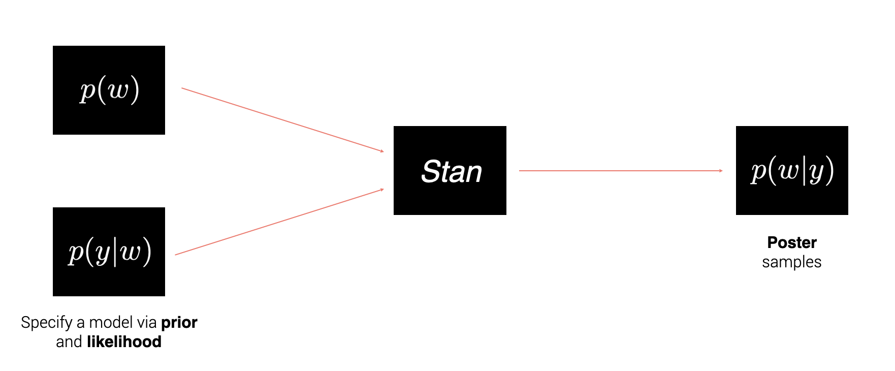
Stan is a probabilistic programming language that implements 2 versions of MCMC: Hamiltonian Monte Carlo (HMC) and the No U-Turn Sampler (or NUTS). NUTS is an improvement over the already great Hamiltonian Monte Carlo and it is the default algorithm used by Stan. I’ve never had a genuine case for using HMC instead of NUTS. Stan also has a python interface called PyStan, so that’s great (and there are also interfaces with other languages).

To work with Stan, one has to specify a likelihood and a prior and Stan will produce samples according the the posterior distribution.

I find this is always better explained with an example, so let’s do that.

Bayesian Logistic Regression in PyStan

So, suppose we’re working on jupyter notebook minding our own business, and we have the variables X and y in memory, which hold the features and labels for the data on figure 1. Now we decide to use logistic regression in a Bayesian way, and we’re going to use Stan for it. The code describing the model will live on it’s own file my_model.stan, and it will look something like this:

Let’s break it down.

1. Stan models are written in blocks. In this case the blocks we’re using are: data (what we know), parameters (what we don’t know) and model (how those 2 things are related).
2. Stan is strongly and statically typed. This means you have to declare the types of your variables before you assign values to them, and the types cannot be changed once declared. Declaring types is necessary because Stan uses C++ templates in the background which makes it very fast. But also, Stan has some built-in types that are very handy when building more complicated models. For instance, if you wish to write a model with 2 parameters, \(w_1\) and \(w_2\) such that \(w_1 < w_2\), one can simply declare such parameter as ordered[2] w and Stan will take care of the rest.
3. The data block. This block tells stan what the given variables will be. Note however, that the data is only being declared. There are no assignments. Assignment happens at a later stage on the Python side of things. Declarations can include constraints, such as <lower=0>. Once we do the assignments, Stan will check that the constraints are satisfied and will throw an exception if that’s not the case.
4. The parameters block. All the unknowns of your model are declared in this block. As with the data block, one can specify constraints in the declarations but these constraints serve a different purpose. Given the constraints, Stan will do some re-parametrization in the background in order to ensure that the constraints are satisfied without having to constraint the parameter space; this makes sampling really efficient.
5. The model block. This is where one writes down the likelihood and the prior. It might sound like a tempting idea to have one block for the likelihood and one block for the priors, but this distinction is not always clear cut. In the end, the prior and likelihood are just factors in the posterior distribution so having them in the same block is simpler.
6. The likelihood. I want to model my data using logistic regression, this means that the likelihood for each data point is given by: \begin{align} y_i \sim \mathrm{Bernoulli}(\mathrm{logit}^{-1}(X_i \cdot w)) \tag{9}\label{eq:nine} \end{align} But I’m taking advantage of Stan’s vectorized notation so that I don’t have to write a for-loop over the index i. Also, you see that instead of writing the likelihood as bernoulli(inv_logit(X * w)), I wrote bernoulli_logit(X * w). Both have the same mathematical meaning but the latter is a numerically stable implementation.
7. And finally the prior. I’m using a normal distribution centered at zero. Like we saw, this is equivalent to an L2 regularisation.

Once our model is ready, we can use it with the pystan library:

Passing the data to the model is pretty simple as you can see. Just make sure that the keys in your data dictionary coincide with the declarations in the data block of the stan file. Once you run the sampling the result you get is like a dictionary, the keys are the parameter names and the values will be the samples produced for the corresponding parameter. The object representation that the Stan developers have chosen contains a nice summary of the sampling:

Inference for Stan model: anon_model_eebce64937b60d5594b9d2238e3ebfe1.
4 chains, each with iter=2000; warmup=1000; thin=1; 
post-warmup draws per chain=1000, total post-warmup draws=4000.

       mean se_mean     sd   2.5%    25%    50%    75%  97.5%  n_eff   Rhat
w[1]   0.18    0.02   0.72  -1.17   -0.3   0.13   0.64   1.73   1385    1.0
w[2]    1.3    0.02   0.59   0.35   0.85   1.22   1.67   2.61   1366    1.0
lp__  -1.91    0.03   1.03  -4.69  -2.27  -1.61  -1.19  -0.95   1079    1.0

Samples were drawn using NUTS at Thu Sep 24 11:39:35 2020.
For each parameter, n_eff is a crude measure of effective sample size,
and Rhat is the potential scale reduction factor on split chains (at 
convergence, Rhat=1).

For each parameter, the summary gives you the mean and its error, the standard deviation, and some percentiles. You also see the columns n_eff and Rhat. A quick explanation about this.

• n_eff: At the very top of the summary, you can see that Stan drew a total of 4000 samples. However, the samples produced by MCMC methods are not independent, they are correlated. What the n_eff column is saying is “For parameter w_1, the 4,000 correlated samples are like having 1,385 independent samples”. You can get more samples via the iter kwarg in the sampling method.
• Rhat: This one is a bit more technical. To generate the samples, MCMC methods explore the distribution of interest using more than one chain. Roughly speaking, if the chains do not agree on what they saw during the exploration, Rhat will be far from 1.0 and you shouldn’t trust the results.

If you want to visualize the full distribution, you can use seaborn to plot a joint distribution:

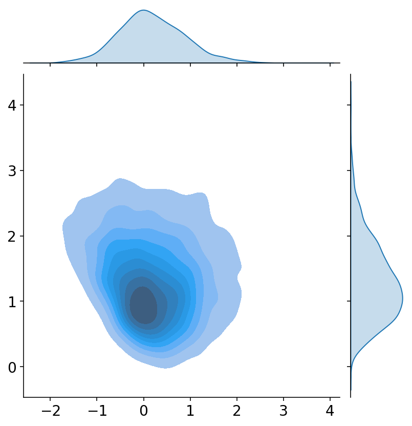
So far, we have only solved the problem of estimating the parameters. If we had to provide a point estimate of our results, the mean column on the summary will be the way to go in most situations. But do not make the mistake of using the mean estimates to make predictions about future data. In the widget below you can check that whichever point you choose on the parameter space, the predictions will have the same issue, namely that the boundary extends on a straight line as we go away from the data.

What you have to do is make use of equation \eqref{eq:eight} and take the average of the predictions (this is not the same as making predictions with the average parameter). When taking the average over several predictions you will see a nice pattern emerging. Each parameter gives a different prediction away from the data, so when you take the average prediction the classification boundary will fan-out! The following piece of code shows you how to do this.

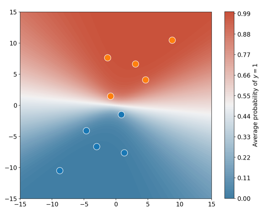
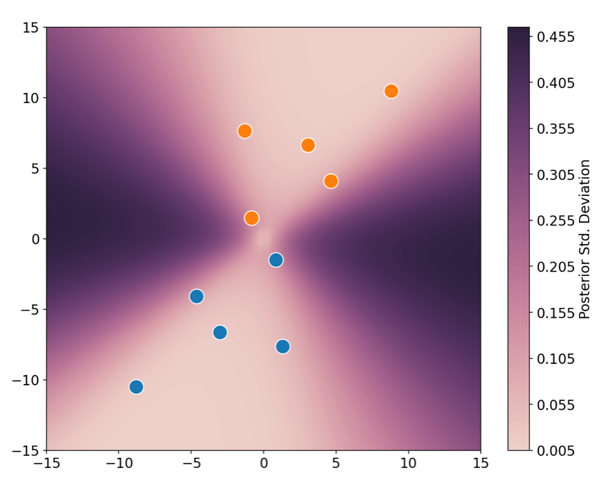
If you have a soul, I expect you appreciate how cool the above plot is. And if that’s not enough, one can also take the standard deviation of the predictions, which essentially places error bars over the predicted probabilities! In this next plot, you can see the regions on which one can/cannot trust the predicted values. As expected, far away from the data the standard deviation is large, so one should take the model’s predictions with a pinch of salt.

Closing remarks

If there’s something about this post that is worth noting, is the amount of stuff I’ve glossed over or ignored. So, if you’re interested in learning more, these are some of the resources I recommend:

• Information theory, inference and learning algorithms by David Mackay. This is the book that establishes machine learning as an inference problem. It’s my personal favorite.
• Data analysis using regression and multilevel/hierarchical models by Andrew Gelman and Jennifer Hill. This book is so under rated. Yes, it is old, and yes it is uses R, and yes it uses BUGS (not Stan), and yes it’s not entirely Bayesian. But this book will give you so much intuition and tricks on how to build models from the ground up! If you’re a complete beginner to modelling, start here. Trust me. The first part of this book has now been updated and it’s available as a separate book called Regression and other stories.
• Bayesian data analysis by Toomanycoolauthors. This is the favorite reference of many people I know so I feel I should recommend it, though I’m personally not it’s biggest fan.
• Mike Betancourt’s blog posts. This is just a great reference for Stan and Bayesian statistics.