Poisson regression in python
You tried to model count data using linear regression and it felt wrong. All your observations are integers and yet your model assumed continuous data. Noise seems to be larger when your observations take large values, but your model assumed the same amount of variance all across the board. Even worse, when your observations take small values, sometimes your model predicted negative values! So when no one else was watching you truncated your predictions at zero, y_pred = max(0, y_pred). You have not slept since then.
Finally, you realise: you need to model your data using a Poisson distribution! After watching a couple of YouTube videos doing some thorough research, you find that every single tutorial and reference out there uses R instead of Python. You’re now considering installing RStudio – but maybe not, since you have a deadline ahead of you and learning a new programming language is not going to happen in one day. Stress is kicking in.
Fear not. Here you will learn how to do Poisson regression, and all within the comfort of your beloved Python. I’ll show you how to model the same example that is treated in chapter 6 of this book1. But, yes, we’ll do it in Python. So fire up a Jupyter notebook and follow along.
Setup
Start by importing the necessary libraries and the data.
You should see a table like this:
| stops | pop | past.arrests | precinct | eth | crime |
|---|---|---|---|---|---|
| 75 | 1720 | 191 | 1 | 1 | 1 |
| 36 | 1720 | 57 | 1 | 1 | 2 |
| 74 | 1720 | 599 | 1 | 1 | 3 |
| 17 | 1720 | 133 | 1 | 1 | 4 |
| 37 | 1368 | 62 | 1 | 2 | 1 |
The data consists of stop and frisk data with noise added to protect confidentiality. This is important because it means that the estimates here will not reproduce the exact same results as in the book or the article. But the lessons of it remain true. Here’s a quick description of the data.
- stops: The number of police stops between January 1998 and March 1999, for each combination of precinct, ethnicity and type of crime.
- pop: The population.
- past.arrests: The number of arrests that took place in 1997 for each combination of precinct, ethnicity and type of crime.
- precinct: Index for the precinct (1-75).
- eth: Indicator for ethnicity, black (1), hispanic (2), white (3). Other ethnic groups were excluded because ambiguities in the classification would cause large distortions in the analysis2.
- crime: Indicator for the type, violent (1), weapons (2), property (3), drug (4).
In a Poisson model, each observation corresponds to a setting like a location or a time interval. In this example, the setting is precinct and ethnicity – we index these with the letter \(i\). The response variable that we want to model, \(y\), is the number of police stops. Poisson regression is an example of a generalised linear model, so, like in ordinary linear regression or like in logistic regression, we model the variation in \(y\) with some linear combination of predictors, \(X\).
\begin{align} y_i &\sim \mathrm{Poisson}(\theta_i) \newline \theta_i &= \exp (X_i \beta) \newline X_i\beta &= \beta_0 + X_{i,1}\beta_1 + X_{i,2}\beta_2 + … + X_{i,k}\beta_k . \end{align} My notation implicitly assumes that \(X_{i, 0} = 1\) for all observations, just so that I don’t have to write the intercept term separately. The use of the exponential in second row is needed because the parameter passed to the Poisson distribution has to be a positive number. The linear combination \(X_i\beta\) is not constrained to be positive, so the exponential is used a link to the allowed paramters. Other choices of link functions are posible but the exponential is the standard choice when it comes to Poisson regression.
The model above would work just fine, but it is most common to model \(y\) as relative to some baseline variable \(u\). This baseline variable is also called the exposure. So, the model we use is written as
\begin{align} y_i \sim \mathrm{Poisson}(u_i \theta_i) = \mathrm{Poisson}(\exp (X_i \beta + \log(u_i))). \end{align} In other words, the logarithm of the exposure plays the role of an offset term.
As in the book, we are going to fit the model in 3 different ways. But before that, we need to put our data in the right shape.
Pretty neat, huh? I learned the above “trick” from a colleague, who in turn says he learned it from this blog. Every processing step takes place in a separate line which makes it easier to read, and your code is not cluttered with multiple assignments to X. We added the column intercept because we will need to pass that explicitly to the statsmodels.api (this step would not be necessary if we were using the statsmodels.formula.api instead, but I’ll not do that here).
Poisson regression
Offset and constant term only
First we fit the model without any predictors, \begin{align} y_i \sim \mathrm{Poisson}(\exp (\beta_0 + \log(u_i))). \end{align}
If you are familiar with scikit-learn, pay attention to how the model here is fitted: the fit method does not operate in place but rather returns a new object storing the results.
That should print the following output:
                 Generalized Linear Model Regression Results
==============================================================================
Dep. Variable:                  stops   No. Observations:                  225
Model:                            GLM   Df Residuals:                      224
Model Family:                 Poisson   Df Model:                            0
Link Function:                    log   Scale:                          1.0000
Method:                          IRLS   Log-Likelihood:                -23913.
Date:                Wed, 20 May 2020   Deviance:                       46120.
Time:                        08:01:45   Pearson chi2:                 4.96e+04
No. Iterations:                     5
Covariance Type:            nonrobust
==============================================================================
                 coef    std err          z      P>|z|      [0.025      0.975]
------------------------------------------------------------------------------
intercept     -0.5877      0.003   -213.058      0.000      -0.593      -0.582
==============================================================================
That table contains a lot of information, but for this tutorial you want to pay attention to 3 fields: the coef and std err of the intercept term (both in the last row), and the Deviance (here equal to 46120). The standard error helps you diagnose if the coefficient found is statistically significant or not. As usual, you’ll want your coefficients to be more than 2 standard errors away from zero. Don’t get hung up on this, though, it is what it is. The deviance is a measure of error, so lower is better. However, adding one meaningless predictor to your model will still make the deviance go down by roughly 1 unit. Thus, as you add parameters to your model, you want to make sure the deviance goes down by more than 1 unit per parameter added.
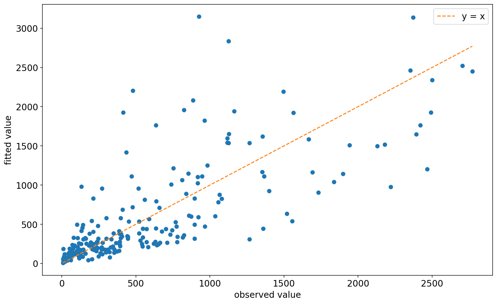
I know what you’re thinking: is that model any good?. Let’s plot the observed values vs the fitted values. The fitted values are conveniently stored in the fittedvalues attribute of the result.
Hmmmm… Perhaps not as bad as I would’ve expected for a 1 parameter model. Still, not the kind of model you bring home to meet your parents. Let’s put some actual features into the model.
Ethnicity and precinct as predictors
We build on top of the previous model by first adding the ethnicity indicators. Note that we don’t add the ethnicity indicator for black (1) because we use it as the baseline.
                 Generalized Linear Model Regression Results
==============================================================================
Dep. Variable:                  stops   No. Observations:                  225
Model:                            GLM   Df Residuals:                      222
Model Family:                 Poisson   Df Model:                            2
Link Function:                    log   Scale:                          1.0000
Method:                          IRLS   Log-Likelihood:                -23572.
Date:                Thu, 21 May 2020   Deviance:                       45437.
Time:                        06:28:28   Pearson chi2:                 4.94e+04
No. Iterations:                     6
Covariance Type:            nonrobust
==============================================================================
                 coef    std err          z      P>|z|      [0.025      0.975]
------------------------------------------------------------------------------
intercept     -0.5881      0.004   -155.396      0.000      -0.596      -0.581
eth_2          0.0702      0.006     11.584      0.000       0.058       0.082
eth_3         -0.1616      0.009    -18.881      0.000      -0.178      -0.145
==============================================================================
Adding the two ethnicity indicators as predictors decreased the deviance by 683 units. Keep in mind that if the ethnicity indicators were just noise, we should expect a decrease in deviance of around 2 units. So this is a good sign. Besides, both coefficients are significant.
Finally, let’s also control for precinct (we use precinct_1 as the baseline).
                Generalized Linear Model Regression Results
==============================================================================
Dep. Variable:                  stops   No. Observations:                  225
Model:                            GLM   Df Residuals:                      148
Model Family:                 Poisson   Df Model:                           76
Link Function:                    log   Scale:                          1.0000
Method:                          IRLS   Log-Likelihood:                -2566.9
Date:                Thu, 21 May 2020   Deviance:                       3427.1
Time:                        06:52:56   Pearson chi2:                 3.24e+03
No. Iterations:                     6
Covariance Type:            nonrobust
===============================================================================
                  coef    std err          z      P>|z|      [0.025      0.975]
-------------------------------------------------------------------------------
eth_2           0.0102      0.007      1.498      0.134      -0.003       0.024
eth_3          -0.4190      0.009    -44.409      0.000      -0.437      -0.401
precinct_2     -0.1490      0.074     -2.013      0.044      -0.294      -0.004
precinct_3      0.5600      0.057      9.866      0.000       0.449       0.671
  ...
precinct_75     1.5712      0.076     20.747      0.000       1.423       1.720
intercept      -1.3789      0.051    -27.027      0.000      -1.479      -1.279
===============================================================================
Check out that massive decrease in the deviance – precinct factors are definitely not noise. As it’s also pointed out in the book, adding precinct factors changed the coefficients for ethnicity. Now we see that the stop rates for black and hispanic are very similar, while whites are 34% less likely to be stopped3.
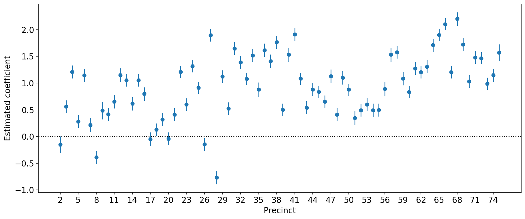
With so many precincts, you might find it easier to see the estimated coefficients in a plot. Let’s do that here.
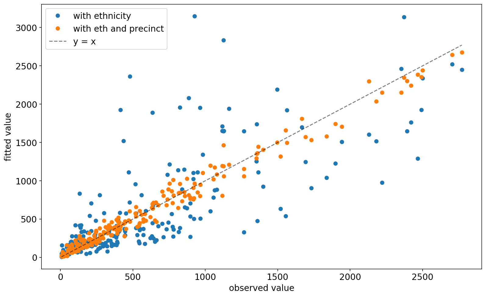
So we see that most coefficients are significant. Finally, if you’re not yet convinced that the precinct factors are good, compare the fitted values of this model vs the fitted values of the model that only uses ethnicity (code not shown):
Overdispersed Poisson
As you might have noticed, the Poisson distribution does not have independent paramter for the variance like, say, a normal distribution. Turns out that for the Poisson distribution, \(y\sim\mathrm{Poisson}(\lambda)\), the variance is equal to the mean. \begin{align} \mathrm{E}\left[y\right] &= \lambda\newline \mathrm{Var}\left[y\right] &= \lambda \end{align}
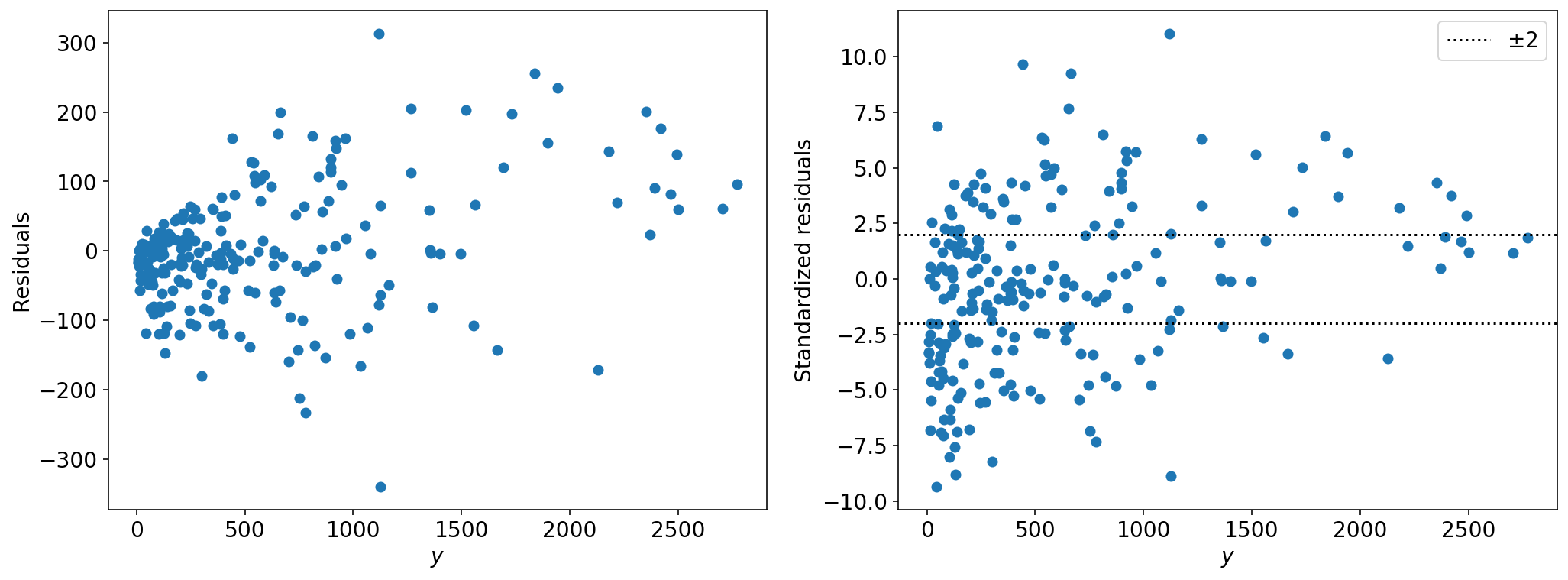
This means that you can easily evaluate if your data is Poisson or not. You already know that the residuals of your fit should have mean equal to zero. We can go a bit further and look at the standardized residuals,
\begin{align} z_i & = \frac{y_i - \mu}{\sigma}\newline & = \frac{y_i - \hat{y}_i}{\sqrt{\hat{y}_i}} \quad \mathrm{(For\ a\ Poisson\ model)} \end{align}
which not only should have mean at zero, but also standard deviation equal to \(1\). The result of statsmodels conveniently stores the values of the residuals and standardized residuals in the attributes resid_response and resid_pearson, so this makes our life a bit simpler:
From the left plot, we see that the variance increases with the fitted values – as expected from a Poisson distribution. But the if the data were well described by our Poisson model, 95% of the standardized residuals should lie within 2 standard deviations. This is obviously not the case. To quantify this, the number you should look at is the overdispersion ratio, \(R\), which is
\begin{align} R = \frac{1}{n - k}\sum_{i=1}^n z_i^2, \end{align}
where \(n-k\) are the degrees of freedom of the residuals (\(n\) is the number of observations and \(k\) is the number of parameters you used to fit the model). If the data were Poisson, the sum of squares of the standardised residuals would follow a chi-square distribution with \(n-k\) degrees of freedom, so we would expect \(R\approx 1\). When \(R > 0\), we say the data is overdispersed because there is extra variation in the data which is not captured by the Poisson model. When \(R < 1\), we say the data is under-dispersed and we make sure to tell all of our friends about it because this is such a rare pokémon to find. You can easily compute the overdispersion ratio from the result:
Ok, so how do we account for overdispersion? There’s more than one way to do it but, in any case, we are going to need an extra parameter in our model (just like a normal distribution has a parameter for the mean and one for the variance). Here, I’ll do it using a negative binomial distribution instead of a Poisson. If \(y\sim \mathrm{NegBinomial}(\mu, \alpha)\), then, according the parametrisation used by statsmodels library,
\begin{align} \mathrm{E}\left[y\right] &= \mu \newline \mathrm{Var}\left[y\right] &= \mu + \alpha\mu^2. \end{align}
The parameter alpha is what helps us to specify the amount of overdispersion. So we simply fit a negative binomial model with a bit of overdisperssion, say \(\alpha=0.051\), (below I explain how to choose this number):
                 Generalized Linear Model Regression Results
==============================================================================
Dep. Variable:                  stops   No. Observations:                  225
Model:                            GLM   Df Residuals:                      148
Model Family:        NegativeBinomial   Df Model:                           76
Link Function:                    log   Scale:                          1.0000
Method:                          IRLS   Log-Likelihood:                -1301.7
Date:                Fri, 22 May 2020   Deviance:                       242.63
Time:                        20:52:46   Pearson chi2:                     231.
No. Iterations:                     9
Covariance Type:            nonrobust
===============================================================================
                  coef    std err          z      P>|z|      [0.025      0.975]
-------------------------------------------------------------------------------
eth_2           0.0086      0.038      0.225      0.822      -0.066       0.083
eth_3          -0.4858      0.039    -12.361      0.000      -0.563      -0.409
precinct_2     -0.2385      0.201     -1.186      0.236      -0.633       0.156
precinct_3      0.5810      0.195      2.983      0.003       0.199       0.963
 ...
precinct_75     1.1591      0.214      5.428      0.000       0.741       1.578
intercept      -1.2272      0.144     -8.545      0.000      -1.509      -0.946
So after accounting for the overdispersion, the standard errors of our coefficients get larger, so it is important that you check which coefficients remain significant. Note that the deviance is calculated differently for the negative binomial model, so do not attempt to compare the deviance of this model with the previous one.
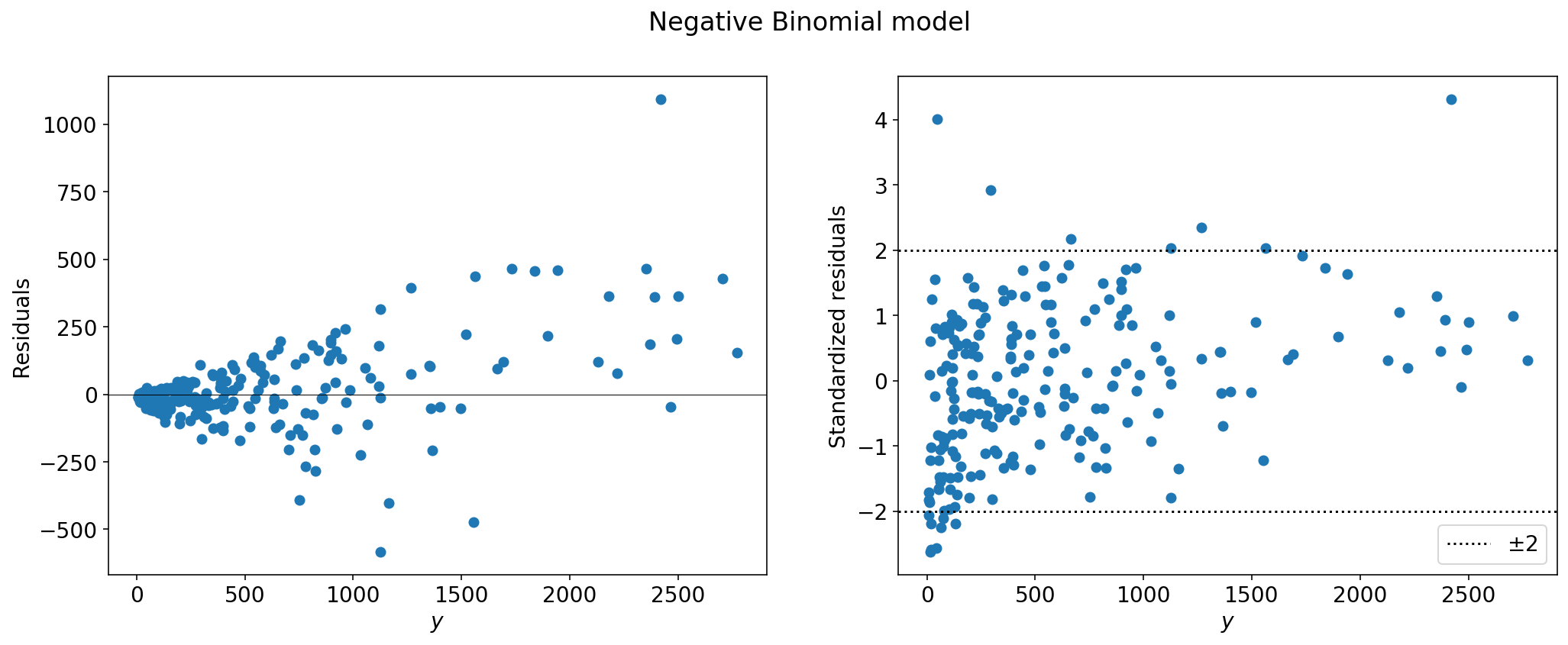
Now take a look at the residuals,
that’s more like it!
Now, how did I choose \(\alpha = 0.0511\). Turns out you can also fit this parameter from the data, but you have to use a different API.
                     NegativeBinomial Regression Results
==============================================================================
Dep. Variable:                  stops   No. Observations:                  225
Model:               NegativeBinomial   Df Residuals:                      148
Method:                           MLE   Df Model:                           76
Date:                Fri, 22 May 2020   Pseudo R-squ.:                  0.1525
Time:                        20:58:23   Log-Likelihood:                -1301.7
converged:                       True   LL-Null:                       -1535.9
Covariance Type:            nonrobust   LLR p-value:                 7.543e-58
==============================================================================
                 coef    std err          z      P>|z|      [0.025      0.975]
------------------------------------------------------------------------------
x1             0.0086      0.038      0.224      0.823      -0.067       0.084
x2            -0.4858      0.040    -12.140      0.000      -0.564      -0.407
 ...
x76            1.1590      0.210      5.526      0.000       0.748       1.570
const         -1.2272      0.145     -8.443      0.000      -1.512      -0.942
alpha          0.0511      0.006      9.130      0.000       0.040       0.062
==============================================================================
The summary for this API is different, the very last row contains the MLE for the parameter \(\alpha\). I personally prefer this API precisely because it allows me to fit the overdispersion parameter using MLE; something that is not possible with the other API (don’t ask me why). The statsmodel.api, however, has the advantage of being similar to the way this topic is presented in Gelman’s book and thus why I dedcided to write this blog using it.
I never said this was going to be as smooth as using R, but hey, at least you’ll hand in your work in time.
-
Data Analysis Using Regression and Multilevel/Hierarchical Models by Andrew Gelman and Jennifer Hill. ↩
-
Andrew Gelman, Jeffrey Fagan & Alex Kiss (2007) An Analysis of the New York City Police Department’s “Stop-and-Frisk” Policy in the Context of Claims of Racial Bias, Journal of the American Statistical Association, 102:479, 813-823, DOI: 10.1198/016214506000001040 ↩
-
You get 34% from the estimated coefficient: \(e^{-0.419} \approx 0.66 = 1 - 0.34\). ↩
