Bayesian Neural Networks with Flax and Numpyro
Flax is a deep learning library built on top of the already amazing Jax. Numpyro is a Bayesian inference library also built on top of Jax. This post will teach you how to combine Flax and Numpyro to obtain MCMC estimates for the parameters of a neural network. I’ll not discuss if Bayesian neural networks are a good idea.
Update: The random_flax_module now available in Numpyro makes the whole process a lot easier, so that defining a custom potential energy function (the approach in this post) is no longer necessary. The syntax for defining a model with a bayesian neural network would be
from numpyro.contrib.module import random_flax_module


def model(n_obs, x, y=None):
    mlp = random_flax_module(
        "mlp",
        MLP([5, 10, 1], (1,)),
        prior={
            "Dense_0.bias": dist.Cauchy(),
            "Dense_0.kernel": dist.Normal(),
            "Dense_1.bias": dist.Cauchy(),
            "Dense_1.kernel": dist.Normal(),
            "Dense_2.bias": dist.Cauchy(),
            "Dense_2.kernel": dist.Normal(),
        },
        # Or, if using the same prior for all parameters, we can do:
        #  prior=dist.Normal(),
        input_shape=(1,),
    )
    sigma = numpyro.sample("sigma", dist.LogNormal())
    with numpyro.plate("obs", n_obs):
        mu = mlp(x).squeeze()
        numpyro.sample("y", dist.Normal(mu, sigma), obs=y)
If for any reason, you still need to implement you own potential energy function. Then the material below might still be helpful.
The problem
Some contributions have been made to Numpyro so that it is now possible run SVI against a neural network defined with Flax (the same is true for Haiku). However, if you naively try to run MCMC following a similar recipe you will fail miserably (it happened to a friend). The recommended solution is to implement your own potential energy function for the NUTS sampler.
The what now? I’m glad you asked.
Sampling with custom potential energy
Here’s what you need to know:
- NUTS is a variant of Hamiltonian Monte Carlo (HMC)
- HMC samples from a probability density by constructing an artificial physical system in which the chains are governed by Hamiltonian dynamics (same as Newton laws but way more pedantic).
- The potential energy of the made-up system is given by the negative of the log-density we wish to sample from.
- You don’t need to worry about the kinetic energy.
Before we continue though, let’s import the tools we’ll need and generate some synthetic data, so that the rest of the code makes sense.
import jax
import jax.numpy as jnp
import numpyro
import numpyro.distributions as dist
from numpyro.infer import MCMC, NUTS

numpyro.set_host_device_count(4)
rng = jax.random.PRNGKey(0)
# --- synthetic data
num_observations = 100
a = 0.3
b = 2.5
s = 0.2
x = jnp.linspace(-1, 1, num=num_observations)
eps = jax.random.normal(jax.random.PRNGKey(1), shape=x.shape)
y = a + jnp.sin(x * 2 * jnp.pi / b) + s * eps

# --- constants we'll use
NUM_CHAINS = 4
MCMC_KWARGS = dict(num_warmup=1000, num_samples=1000, num_chains=NUM_CHAINS)
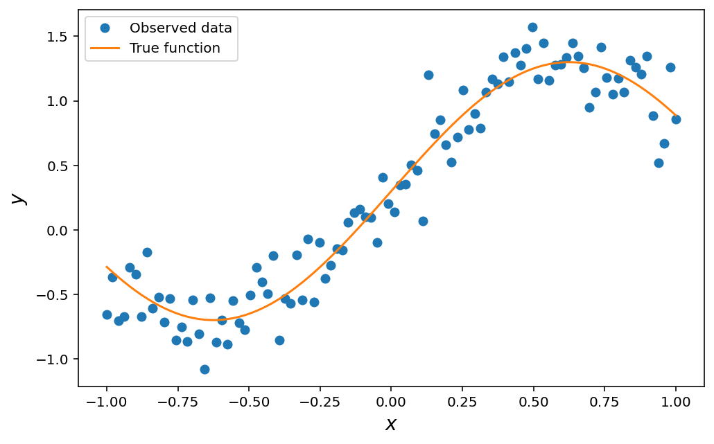
The data we’ve created should look like this:
Usually, we write our models in Numpyro by writing a function of our data. The body of our model function contains a bunch of numpyro.sample statements that tell Numpyro how each parameter in our model is distributed. For example, a linear regression model might look like this:
def linear_regression(x, y=None):
    alpha = numpyro.sample("alpha", dist.Normal())
    beta = numpyro.sample("beta", dist.Normal())
    sigma = numpyro.sample("sigma", dist.LogNormal())

    # --- likelihood
    mu = alpha + beta * x
    numpyro.sample("y", dist.Normal(mu, sigma), obs=y)

kernel = NUTS(linear_regression)
mcmc = MCMC(kernel, **MCMC_KWARGS)
# mcmc.run(key, x, y) ...
Calling NUTS on the linear_regression model looks at the body of the function and builds a joint log-density for all the parameters in the model (here the parameters are alpha, beta, sigma). This joint density is then flipped upside down and used as potential energy for the chains in the sampler. But the NUTS sampler as implemented in Numpyro allows a second, alternative API - by passing your potential function directly. Let’s write the above model as a potential function. I will first write a quick, dirty implementation and I’ll later refine it into something that is easier to generalize. Remember, the potential energy is just the negative of the joint log-density.
def linear_regression_potential(parameters, x, y):
    alpha, beta, sigma = parameters
    # --- priors
    log_prob = (
        dist.Normal().log_prob(alpha)
        + dist.Normal().log_prob(beta)
        + dist.LogNormal().log_prob(sigma)
    )
    # --- likelihood
    mu = alpha + beta * x
    log_likelihood = dist.Normal(mu, sigma).log_prob(y).sum()
    return - (log_prob + log_likelihood)
The above function takes an array of values, parameters, that represent the current value of each parameter and returns the negative of the (unnormalized) joint log-density as defined by our priors and likelihood. Notice how there’s a natural separation in the body of our function because all of our parameters are given independent priors. We’ll use this separation to clean up our code in the next section. However, separate from the fact that it could be written more nicely, this function also depends on x and y which are not parameters in the model. So the potential function is not yet in the form that we need it.
To construct a function that depends only on the model parameters, we “freeze” the values of x and y to the values we’ve already observed (our given data). The resulting function can then be used with the NUTS sampler by explicitly using the keyword argument potential_fn.
from functools import partial

potential = partial(linear_regression_potential, x=x, y=y)
kernel = NUTS(potential_fn=potential)
mcmc = MCMC(kernel, **MCMC_KWARGS)
Now comes a crucial step. To be able to mcmc.run, we need to provide initial values for each of the parameters. We must provide initial values in a way that is compatible with the signature of our potential function. Note how, in the function above, the potential function expects a single array of values and the body of the function will take care of unpacking it in the right way (this is not robust and we’ll fix it in the next section). A common point of confusion when providing the initialization for each parameter is that we must in fact initialize every chain in our sampler. The chain dimension should be the leading dimension in whatever array of initial values we provide. For this example, our potential function expects an array with 3 values (one for each parameter), so the initialization values should have shape (4, 3) because we are using 4 chains. Ideally, every chain would be initialized from a slightly different location but, for now, let’s initialize every chain at the same point. Again, this is something we will fix in the next section. Given the priors I’ve defined on my parameters, I’d say the following is a sensible initialization:
# alpha starts at 0.0, beta at 0.0, sigma at 1.0
single_chain_init = jnp.array([0.0, 0.0, 1.0])
init_params = jnp.tile(single_chain_init, (NUM_CHAINS, 1))
With this, we can finally run our mcmc:
rng, _ = jax.random.split(rng)
mcmc.run(rng, init_params=init_params)
The above sampling should’ve run just fine but the samples are a bit awkward to use. For instance, if you look at mcmc.print_summary() you’ll see somthing like this:
                mean       std    median      5.0%     95.0%     n_eff     r_hat
Param:0[0]      0.29      0.03      0.29      0.24      0.35   3989.05      1.00
Param:0[1]      1.24      0.06      1.24      1.14      1.34   3710.43      1.00
Param:0[2]      0.34      0.02      0.34      0.30      0.38   3639.55      1.00

Number of divergences: 0
Naturally, numpyro doesn’t know how each of your parameters is named. But it’s not just the diagnostics. The fact that our parameters do not have names of their own might not seem like a big deal for this simple linear regression model – we can easily figure out which samples are for alpha, which for beta and which for sigma. But doing this for a neural network will be impractical, to say the least.
This next section will take care of solving the issues we’ve created along the way.
Re-usable logic & nicely structured samples
We now know how sampling with a custom potential works, but there are 3 tasks we need to address
- Write our code with re-usable logic,
- Obtain nicely structured samples,
- Provide different (and sensible) initializations for each chain.
To solve our first two problems, it’s useful to know that the argument we feed to our potential function can in fact be of any type. The samples produced by numpyro will maintain the structure of such type. For example, the potential function in the previous section was a function of a jnp.ndarray, so the samples came out as a jnp.ndarray. But if we write our potential function in such a way that it takes a dictionary (or any mapping) as an argument, then the samples will be given to us in the form of a dictionary. To solve the 3rd problem I will initialize each parameter to a random sample from its prior. This will give me different starting points for each chain, but the constraints of each parameter will not be broken (for example, if my parameter has a log-normal prior, I wouldn’t want to initialize it to a negative value as this would be inconsistent with the log-normal distribution.)
So here’s the solution I came up with. There are probably nicer ways of doing this, but this is the solution that works for me. At least for now. I will specify my models with 3 ingredients:
- A dictionary of prior distributions
- A log-likelihood function
- A dictionary of parameter shapes
Ingredients 1 and 2 will be used to construct the potential function, while ingredients 1 and 3 will be used for the initialization of the chains. As we’ll see in the next section, I can easily obtain those 3 ingredients for a neural network defined with flax. So let’s clean up the code for our linear regression potential. My ingredients 1 and 2 are:
priors = {
    "alpha": dist.Normal(),
    "beta": dist.Normal(),
    "sigma": dist.LogNormal(),
}

def linear_regression_log_likelihood(values: dict, x: jnp.ndarray, y: jnp.ndarray):
    alpha = values["alpha"]
    beta = values["beta"]
    sigma = values["sigma"]
    mu = alpha + beta * x
    return dist.Normal(mu, sigma).log_prob(y)
With these ingredients, I can now construct the potential function.
def evaluate_densities_at_values(densities: dict, values: dict):
    evaluate = lambda values, density: density.log_prob(values)
    return jax.tree_multimap(evaluate, values, densities)


def linear_regression_potential_v2(
    parameter_values: dict,
    parameter_priors: dict,
    x: jnp.ndarray,
    y: jnp.ndarray,
):
    # -- priors
    logprobas = evaluate_densities_at_values(
        parameter_priors,
        parameter_values,
    )
    logprobas, _ = jax.flatten_util.ravel_pytree(logprobas)

    # -- likelihood
    log_likelihood = linear_regression_log_likelihood(
        parameter_values,
        x,
        y,
    )
    # potential
    return -(logprobas.sum() + log_likelihood.sum())

# freeze the priors and the observed data
potential = partial(
    linear_regression_potential_v2,
    parameter_priors=priors,
    x=x,
    y=y,
)
kernel = NUTS(potential_fn=potential)
mcmc = MCMC(kernel, **MCMC_KWARGS)
The first function, evaluate_densities_at_values, helps me to quickly evaluate the densities for all my parameters. In particular, the part of my potential function that requires me to evaluate the prior log-densities will be reusable regardless of my model1.
The 3rd ingredient, shapes, is quite trivial in this case because all my parameters are scalars, so I end up with simply
shapes = {
    "alpha": (),
    "beta": (),
    "sigma": (),
}
And here is how I’d use this ingredient to provide initial values for my chains.
def make_rng_tree(rng, tree, is_leaf=None):
    """
    Provide a random seed for each leaf in the tree.
    """
    # hack because jax.tree_structure does not allow a `is_leaf` kwarg.
    raw_tree = jax.tree_map(lambda x: 1, tree, is_leaf=is_leaf)
    structure = jax.tree_structure(raw_tree)
    subkeys = jax.random.split(rng, structure.num_leaves)
    iter_subkeys = iter(subkeys)
    return jax.tree_map(lambda x: next(iter_subkeys), raw_tree)

def init_to_sample(rng,
    parameter_shapes,
    parameter_densities,
    num_chains=NUM_CHAINS
):
    parameter_seeds = make_rng_tree(
        rng,
        parameter_densities,
        is_leaf=lambda x: isinstance(x, dist.Distribution)
    )
    sample_ = lambda d, s, k: d.sample(k, sample_shape=(num_chains, *s))

    return jax.tree_multimap(
        sample_,
        parameter_densities,
        parameter_shapes,
        parameter_seeds,
        is_leaf=lambda x: isinstance(x, dist.Distribution)
    )

rng, init_rng, mcmc_rng = jax.random.split(rng, 3)
init_params = init_to_sample(init_rng, shapes, priors)
All I’m doing is drawing a sample from the prior distribution for each parameter. The code is slightly complex because I wanted to make something that I can re-use regardless of the data structure I use to define the priors. This is important because, as we’ll see, in a neural network I will use nested dictionaries.
And now that we have it all in place, we can run our mcmc:
mcmc.run(mcmc_rng, init_params=init_params)
mcmc.print_summary()
                mean       std    median      5.0%     95.0%     n_eff     r_hat
     alpha      0.29      0.03      0.29      0.24      0.35   3518.60      1.00
      beta      1.24      0.06      1.24      1.14      1.34   4396.45      1.00
     sigma      0.34      0.02      0.34      0.30      0.38   3694.10      1.00

Number of divergences: 0
Tada!
Let’s now move on to the reason we’re here in the first place.
Bayesian neural network
For context, this is how a simple fully connected network would look like in Flax:
import flax.linen as nn

# Not the final implementation:
class MLP(nn.Module):
    layers: list

    @nn.compact
    def __call__(self, x):
        for num_features in self.layers[:-1]:
            x = nn.softplus(nn.Dense(num_features)(x))
        x = nn.Dense(layers[-1])(x)
        return x
We need a way of translating this model into a potential function. Remember that the logic we developed in the previous section asks for 3 ingredients: priors, shapes, and a log-likelihood function. This might feel like a tedious task but it’s very simple. We are going to take advantage of Flax’s API and the tools we’ve developed so far. I’m going to be using L2 regularization, that is to say, all the parameters in my network will be given a standard normal prior. This is how my actual MLP is going to look like:
class MLP(nn.Module):
    layers: list
    input_shape: tuple

    @nn.compact
    def __call__(self, x):
        for num_features in self.layers[:-1]:
            x = nn.softplus(nn.Dense(num_features)(x))
        x = nn.Dense(layers[-1])(x)
        return x

    def get_priors(self):
        """
        L2 Regularisation
        """
        structure = self._random_init()["params"]
        priors = jax.tree_map(lambda x: dist.Normal(), structure)
        return priors

    def get_shapes(self):
        init = self._random_init()["params"]
        return jax.tree_map(lambda x: x.shape, init)


    def _random_init(self):
        rng = jax.random.PRNGKey(0)
        return self.init(rng, jnp.ones(self.input_shape))
The key methods are get_priors and get_shapes. In both cases, I’m using the fact that the init method of my network creates a pytree with the parameters of the network – I can use that tree to read the correct shapes for each layer and to create a dictionary of prior densities and that’s what these methods do.
The log-likelihood function is quite simple because flax already gives me an apply method for my neural network, so I won’t bother defining a separate function. The only thing to add is that I need to include a noise parameter that is not part of the neural network architecture. This will be a scalar parameter with a log-normal prior again.
output_shape = (1,)
input_shape = (1,)
layers = [5, 10, *output_shape] # Yes, it's a very small MLP.
mlp = MLP(layers, input_shape)

mlp_priors = mlp.get_priors()
other_priors = {"sigma": dist.LogNormal()}
# --- combine all parameters
priors = {**mlp_priors.unfreeze(), **other_priors}
Now we can construct the potential function
def mlp_potential(
    parameter_values: dict,
    parameter_priors: dict,
    apply_fn: callable,
    x: jnp.ndarray,
    y: jnp.ndarray,
):
    log_prior = evaluate_densities_at_values(
        parameter_priors,
        parameter_values,
    )
    log_prior, _ = jax.flatten_util.ravel_pytree(log_prior)
    mu = apply_fn({"params": parameter_values}, x).squeeze()
    log_likelihood = dist.Normal(mu, parameter_values["sigma"]).log_prob(y)
    return -(log_prior.sum() + log_likelihood.sum())

# Freeze the data/known
potential = partial(
    mlp_potential,
    parameter_priors=priors,
    apply_fn=mlp.apply,
    x=x.reshape(-1, 1),
    y=y
)
kernel = NUTS(potential_fn=potential)
mcmc = MCMC(kernel, **MCMC_KWARGS)
Before running the sampler, we will need the initialization for each parameter (and for all chains). Providing initializations based on samples from the priors is straightforward with the code we’ve written.
mlp_shapes = mlp.get_shapes()
other_shapes = {"sigma": ()}
shapes = {**mlp_shapes.unfreeze(), **other_shapes}
rng, init_rng, mcmc_rng = jax.random.split(rng, 3)
init_params = init_to_sample(rng, shapes, priors)
And we can now run the sampler!
mcmc.run(mcmc_rng, init_params=init_params)
Diagnostics & Predictions
We’ve managed to run MCMC on our neural network, but now we want to evaluate if the chains have mixed properly. Unfortunately, if you run mcmc.print_summary() you’ll see a nasty
AttributeError: 'dict' object has no attribute 'shape'
This happens because the samples we’ve obtained contain nested dictionaries and the logic for constructing the summary string breaks down. The nested dictionaries are of course intentional, we do this to reflect the architecture of our neural network. The print_summary logic breaking down is an unintended consequence, but we can still read the diagnostics using jax.tree_map. For example, to check r-hats we can do:
samples_by_chain = mcmc.get_samples(True)
diagnostics = jax.tree_map(
    numpyro.diagnostics.gelman_rubin,
    samples_by_chain,
)
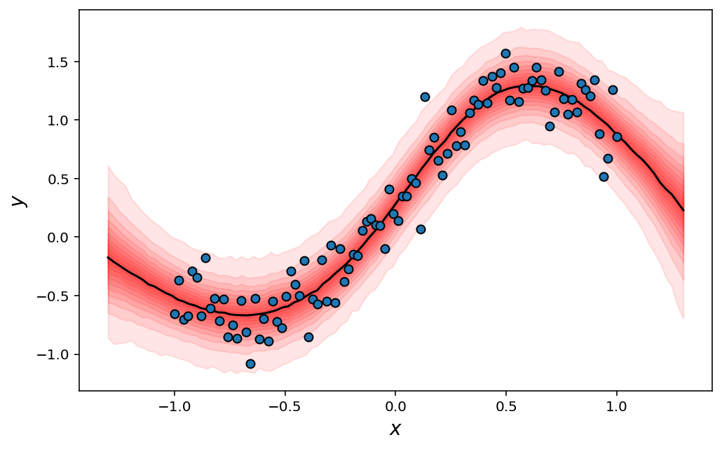
Finally, to construct our predictive distribution, we need to make predictions on our data for every sample we drew. Rather than relying on a slow for-loop implementation, the right approach here is again to make use of Jax’s vmap function, which will be way faster.
x_pred = jnp.linspace(-1.3, 1.3, num=100) # Original data range was (-1, 1)
predict_fn = jax.vmap(
    lambda sample: mlp.apply({"params": sample}, x_pred.reshape(-1, 1)).squeeze(),
)
mu_samples = predict_fn(mcmc.get_samples()) # The network autmatically ignores the parameter `sigma`
sigma_samples = mcmc.get_samples()["sigma"]
y_pred = dist.Normal(mu_samples, sigma_samples.reshape(-1, 1)).sample(rng)
And finish with a fancy plot
Watermark
Author: Omar Sosa Rodriguez

Python implementation: CPython
Python version       : 3.8.10
IPython version      : 7.29.0

Compiler    : Clang 13.0.0 (clang-1300.0.29.3)
OS          : Darwin
Release     : 21.0.1
Machine     : arm64
Processor   : arm
CPU cores   : 10
Architecture: 64bit

matplotlib: 3.4.3
flax      : 0.3.6
jax       : 0.2.24
numpy     : 1.21.4
numpyro   : 0.8.0
-
Almost regardless of my model. ↩